Application Note: Blob Analysis#
You learn how to use the Blob Analysis operators in combination with other operators in VisualApplets. The examples use the Blob Analysis operators for basic object detection and classification inside the FPGA. A line applet shows the use of the Blob Analysis 1D operator. Furthermore, C++ SDK projects for the given examples are available. They allow an understanding of the interpretation of Blob Analysis results on PC side. (Application Note SAN011)
The following design examples illustrate the use of the VisualApplets blob analysis operators:
- Simple Blob Analysis Application Including SDK Project for Object Visualization: This example uses the Blob Analysis for basic object detection. All detected objects are transferred to the host PC.
- Using the Blob Analysis for Classification and ROI Selection: This example shows the use of the Blob Analysis for object detection and classification inside the FPGA.
- Blob Analysis 1D: This example explains the use of the Blob Analysis 1D operator for endless line scan images.
Simple Blob Analysis Application Including SDK Project for Object Visualization#
The first example is a basic Blob Analysis applet. A camera image is binarized. Next, the binary image is send to DMA in path and on the other path a Blob Analysis is performed and the results are output via a second DMA channel.
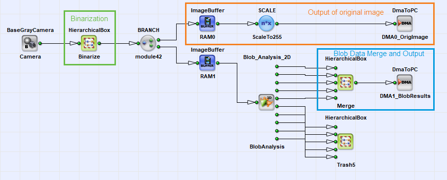
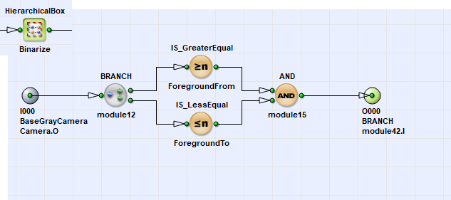
The binarization used in this example is based on simple thresholding. The Blob Analysis assumes every white pixel to be an object pixel. Figure 2 shows that a foreground value range is selected using two threshold values. This allows the use of images where the objects are formed by dark pixels or images where objects are brighter in contrast to their background. After the binarization itself the image is buffered. From the buffer, the images are passed to the Blob Analysis and are transferred to the host PC to monitor the binarized images.
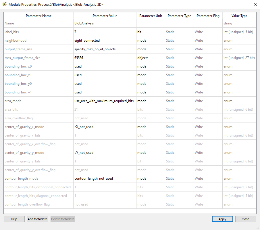
The configuration of the Blob Analysis parameters can be seen in the following figure:
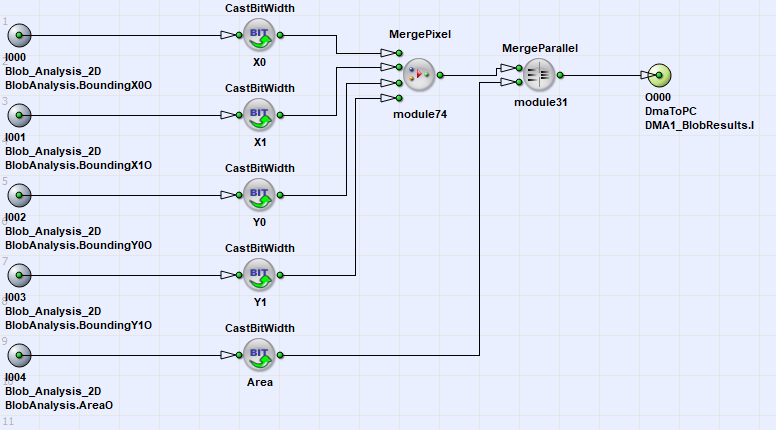
In the image above you see how the Blob Analysis data is merged into one link only. In this example, the features Bounding Box and Area are used. First, the bounding box links of 16Bits each are merged together which results in a link width of 64 Bits. The area is extended to 64Bits as well. Using the InsertPixel operator, both links are merged together. The resulting DMA transmission will therefore be of the following format:
Blob DMA Byte Order for Simple Blob2D Applet#
| Byte No. | Object Feature |
|---|---|
| 0 to 1 | Bounding Box X0 |
| 2 to 3 | Bounding Box X1 |
| 4 to 5 | Bounding Box Y0 |
| 6 to 7 | Bounding Box Y1 |
| 8 to 15 | Area |
Note the varying byte order in the PC. The object features bit widths are extended. In real, the Bounding Box uses 10Bits only to represent the values between 0 and 1023 and the Area uses 21Bits only. A small SDK C++ project is attached to this applet to show its functionality. It can be found together with the design file in folder Examples\Processing\BlobAnalysis\Blob2D of the VisualApplets installation path.
Using the Blob Analysis for Classification and ROI Selection#
This example shows an approach to cut out a region of interest based on extracted object features. The aim is to find the object with the maximum area and to extract the center of gravity of this object used to form the ROI.
The example shows the capability of Visual Applets to use the Blob Analysis results for classification inside the applet which allows a significant enhancement of image processing possibilities inside the frame grabber. Figure 1 shows a screenshot of the design. The main parts are the binarization, the Blob Analysis, the classification and the cut-out of the ROI. These parts will be explained in detail in the following.
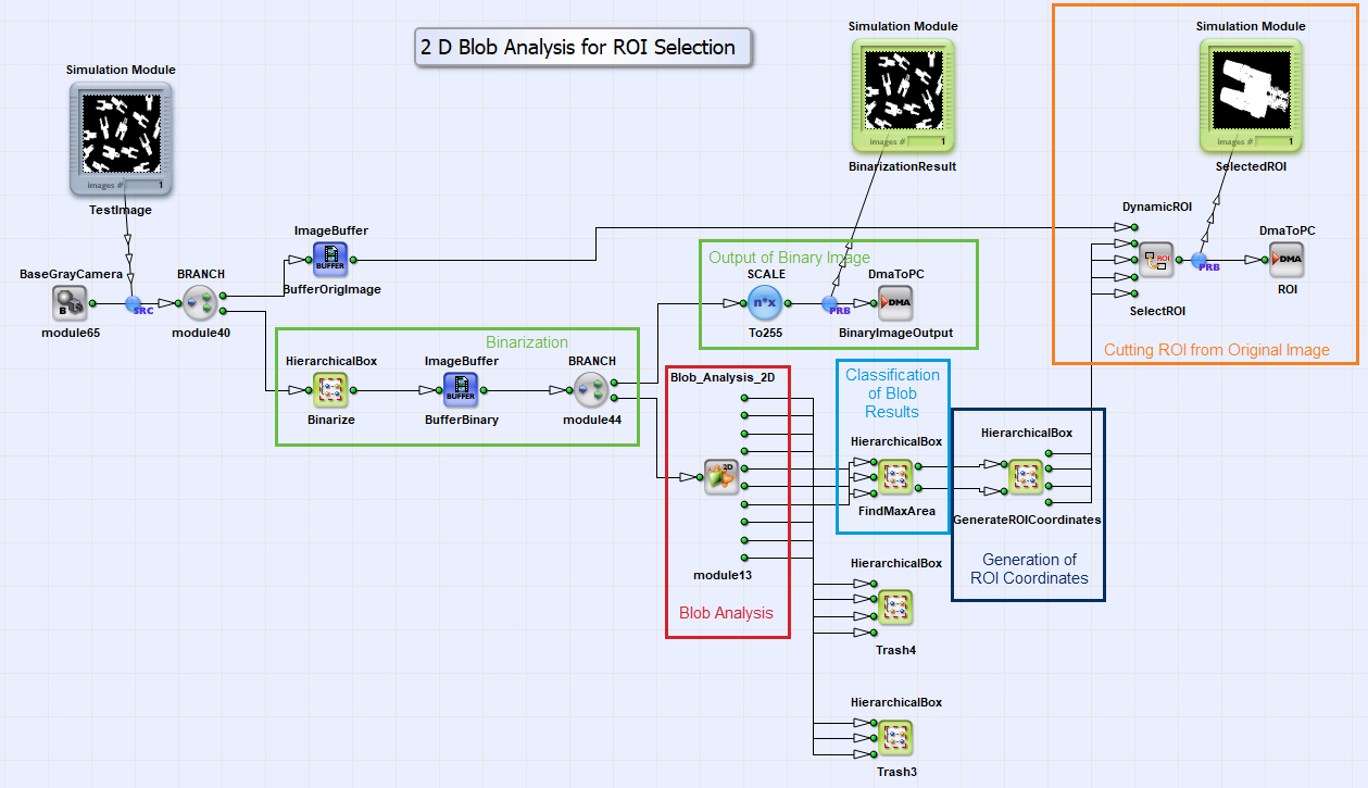
The binarization used in this example is based on simple thresholding. The Blob Analysis assumes every white pixel to be an object pixel. Figure 2 shows that a foreground value range is selected using two threshold values. This allows the use of images where the objects are formed by dark pixels or images where objects are brighter in contrast to their background. After the binarization itself the image is buffered. From the buffer, the images are passed to the Blob Analysis and are transferred to the host PC to monitor the binarized images.
The Blob Analysis is performed post to the binarization. Here, only the object features center of gravity in x and y-direction as well as the area are used for further processing. All other features are not used in this example.
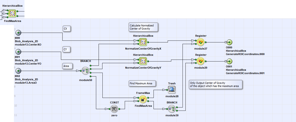
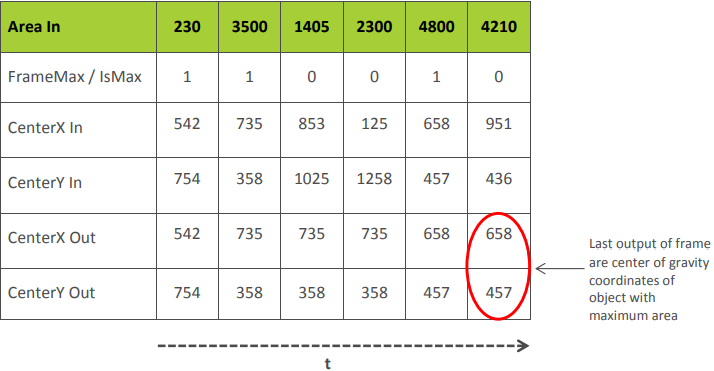
The applet continues with the classification of the Blob Analysis results (Figure 3). First, the center of gravity values are normalized by dividing them with the area. This is simply done by using the DIV operator. Meanwhile the detection of the object with the largest area is performed. Here, the operator FrameMax and Registers are used. The idea of the classification algorithm is to suppress every object whose area is less than the objects which have been investigated so far. In detail, the Blob Analysis outputs a stream of objects. The FrameMax operator detects if a current object is larger than the objects which have been investigated so far and outputs logic one at its output IsMax.This value is used at the Capture input of the registers. If the current object is larger than the previous objects the center of gravity coordinates are latched to the output. Hence, the last output of the frame i.e. the blob stream represents the center of gravity coordinates of the object which has the maximum area. Figure 3 illustrates this behavior.
The classification module now outputs the center of gravity coordinates of the largest object found in the image. Next, the coordinates have to be transformed to the ROI coordinates XOffset, XLength, YOffset and YLength. Figure 4 shows the design of this transformation. The XLength and YLength is set to a constant whereas the center of gravity coordinates are reduced by half of the ROI size.
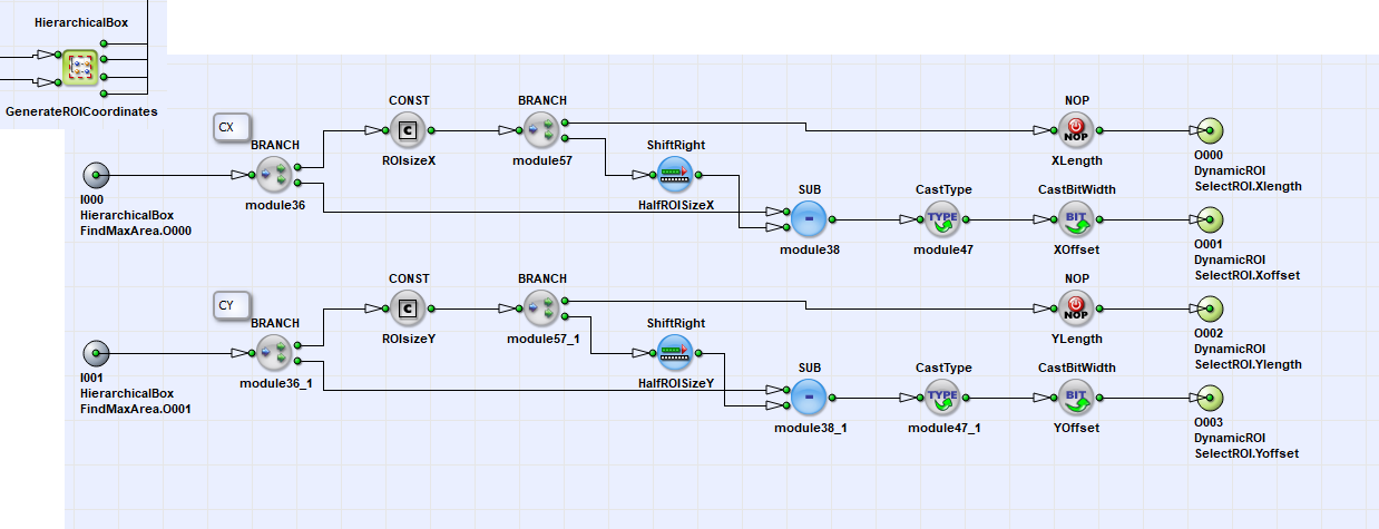
The four ROI values are now used to cut-out the ROI from the original image using the DynamicROI operator. As explained previously the classification module outputs the object with the maximum area with the last value of the frame. This is favorable as the DynamicROI operator only considers the last ROI coordinates received. Hence, the correct coordinates are used and the largest object is cut-out from the original image. The design file of this VisualApplets project can be found in folder Examples\Processing\BlobAnalysis\Blob2D_ROI_select in the VisualApplets installation path. The applet can be run in microDisplay and the results can directly be seen. Moreover, a small SDK project is added to the example. To use the SDK project it is required to change the DMA size of the ROI to the DMA size set by modules ROIsizeX and ROIsizeY. Use the display settings in microDisplay or the widht1 and height1 parameters in the SDK project to perform the adaptation.
Blob Analysis 1D#
The Blob Analysis 1D example illustrates the use of the 1D blob operator in a VisualApplets environment.
The 1D Blob Analysis example is a simple applet based on a base line camera. The camera is used with a line trigger only. Hence, the applet is based on real 1D images. For DMA transmission, the original image is transformed into small pieces of successive lines forming a 2D image. All parts of the applet will be explained in detail in the following. Figure 1 shows the main sheet of the design.
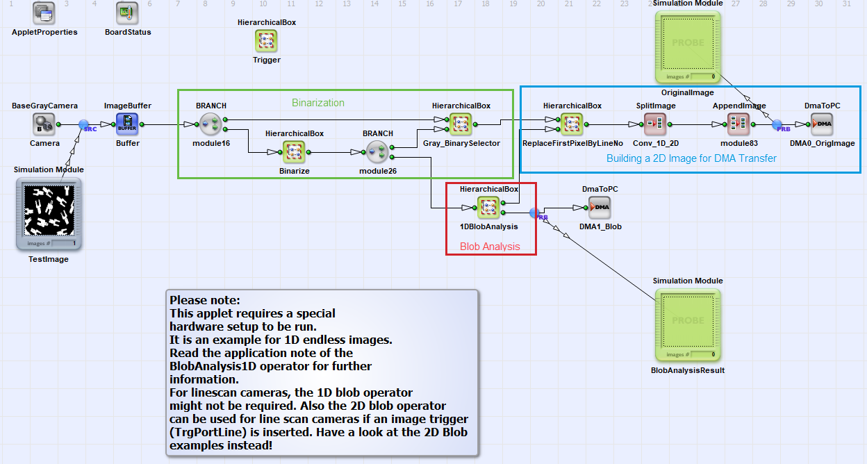
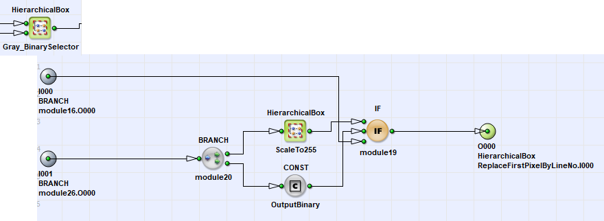
For acquisition, a line camera operator connected to an ImageBuffer is used. This buffer allows the buffering of 1D image lines. Next, in the Hierarchical Box Binarize a simple thresholding is performed to convert the pixels into foreground and background pixels. A selector allows switching the original image and the binary image to the image output path. This is simply done by an IF operator and a CONST operator. The dynamic parameter of the CONST operator allows the modification of the IF operator's condition input to switch its inputs. Hence, during runtime it is possible to switch between the original grayscale image and the binarized image.
As the applet's application purpose will be the visualization of the objects found in the original image it is required to allow a synchronization of both DMA channels in the PC. A line marker is used to mark every line of the original image and every blob. Hence a counter is used to count every line. The line counter is contained in the Hierarchical Box 1DBlobAnalysis together with the blob analysis operator and the line count value leaves the box through the upper link O000. The counter has a range of 10 bits. Hence, an overflow occurs at value 1024 and the counter starts from zero again.
In ReplaceFirstPixelByLineNo the first four pixels of a line are replaced by the line count. For that purpose the parallelism is changed so operation is done at a granularity of 32 bit. The x-coordinate is count and every time the x-coordinate is zero, the line number (expanded to 32 bit) is forwarded instead of the original pixel values.
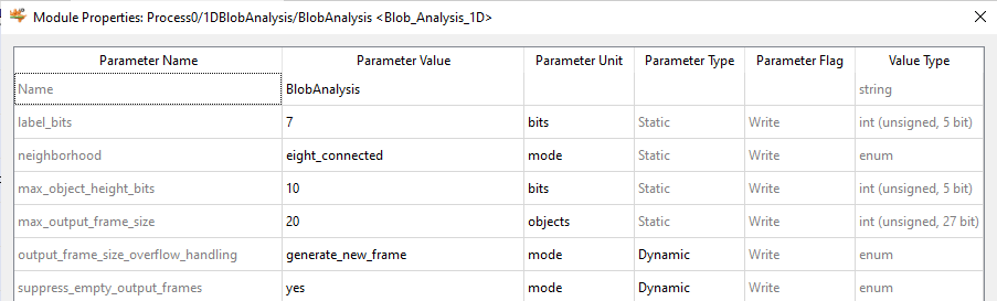
Beside the line marker it is required generating a flush condition for the Blob Analysis operation. The flush may be implemented as a trigger input or in this case, a flush condition is produced once every line. Hence, the Blob Analysis will finalize (Eof) its output once a line. However, the Blob Analysis is configured to this behavior only if the output frame is not empty by using parameter supres_empty_output_frames. Furthermore, the Blob Analysis is configured to a maximum object height of 10 bits i.e., 1024 pixels. The maximum output frame size of the operator is set to 20. If more objects have to be output and no flush condition occurs, the operator will generate a new frame. These small output frames allow a minimization of the time the object has been detected and the time it can be analyzed in the PC.
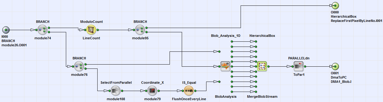
The 11 Blob Analysis output streams are merged into one stream which is connected to the DMA. This is simply done using MergePixel and InsertPixel operators. The order of the object features is shown in the table below.
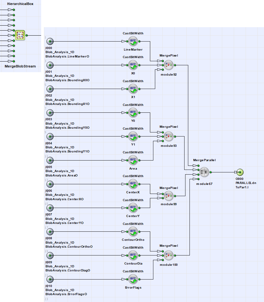
| Byte No. | Object Feature |
|---|---|
| 0 to 3 | Line Marker |
| 4 to 5 | Bounding Box X0 |
| 6 to 7 | Bounding Box X1 |
| 8 to 11 | Center of Gravity Y |
| 12 to 15 | Center of Gravity Y |
| 16 to 17 | Bounding Box Y0 |
| 18 to 19 | Bounding Box Y1 |
| 20 to 23 | Area |
| 24 to 25 | Contour Length Diagonal |
| 26 to 27 | Contour Length Orthogonal |
| 28 to 31 | Error Flags |
The run of this project in hardware requires a special hardware setup with line camera and trigger encoder system. The design file can be found in folder Examples\Processing\BlobAnalysis\Blob1D in the Visual Applets installation path. A complex SDK project is added to the design which mostly demonstrates the displaying of objects.